반응형
yunjey/pytorch-tutorial
PyTorch Tutorial for Deep Learning Researchers. Contribute to yunjey/pytorch-tutorial development by creating an account on GitHub.
github.com
네이버 최윤제님의 자료를 통해 공부하고 기록한 글입니다.
파이토치를 통해 GAN을 구현하고, MNIST 데이터 셋을 이용해 실습했습니다.
Google Colab 을 사용했습니다.
라이브러리 불러오기 및 하이퍼파라미터 설정
import torch
import torch.nn as nn
import torch.optim as optim
import torchvision.utils as utils
import torchvision.datasets as dsets
import torchvision.transforms as transforms
from torchvision.utils import save_image

import os
import numpy as np
import matplotlib.pyplot as plt
device = 'cuda' if torch.cuda.is_available() else 'cpu'
print(f"device = {device}")
sample_dir = 'samples'
if not os.path.exists(sample_dir):
os.makedirs(sample_dir)# 하이퍼파라미터 설정
latent_size = 64
hidden_size = 256
image_size = 784 # 28 * 28
num_epochs = 300
batch_size = 100MNIST DATASET
# Image Processing
transform = transforms.Compose([
                    transforms.ToTensor(),
                    transforms.Normalize(mean=[0.5], # 1 for gray scale 만약, RGB channels라면 mean=(0.5, 0.5, 0.5)
                                         std=[0.5])])  # 1 for gray scale 만약, RGB channels라면 std=(0.5, 0.5, 0.5)

# MNIST 데이터셋
mnist_train = dsets.MNIST(root='data/',
                         train=True, # 트레인 셋
                         transform=transform,
                         download=True)
mnist_test  = dsets.MNIST(root='data/',
                          train=False,
                          transform=transform,
                          download=True)
# 랜덤으로 9개만 시각화
figure = plt.figure(figsize=(8, 8))
cols, rows = 3, 3
for i in range(1, cols * rows + 1):
sample_idx = torch.randint(len(mnist_train), size=(1,)).item()
img, label = mnist_train[sample_idx]
figure.add_subplot(rows, cols, i)
plt.axis("off") # x축, y축 안보이게 설정
plt.imshow(img.squeeze(), cmap="gray")
plt.show() 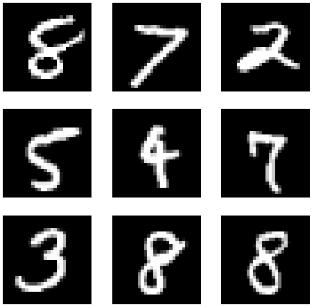
Data Loader
# 데이터 로더
data_loader = torch.utils.data.DataLoader(dataset=mnist_train, # 훈련용 데이터 로딩
                                          batch_size=batch_size,
                                          shuffle=True) # 에폭마다 데이터 섞기
생성자 G 와 판별자 D
# Discriminator
D = nn.Sequential(
    nn.Linear(image_size, hidden_size),
    nn.LeakyReLU(0.2),
    nn.Linear(hidden_size, hidden_size),
    nn.LeakyReLU(0.2),
    nn.Linear(hidden_size, 1),
    nn.Sigmoid()) # Binary Cross Entropy loss 를 사용할 것이기에 sigmoid 사용!

# Generator
G = nn.Sequential(
    nn.Linear(latent_size, hidden_size),
    nn.ReLU(),
    nn.Linear(hidden_size, hidden_size),
    nn.ReLU(),
    nn.Linear(hidden_size, image_size),
    nn.Tanh())

# Device setting
D = D.to(device)
G = G.to(device)
def imshow(img):
img = (img+1) / 2
img = img.squeeze() # 차원 중 사이즈 1 을 제거
np_img = img.numpy() # 이미지 픽셀을 넘파이 배열로 변환
plt.imshow(np_img,cmap='gray')
plt.show()
def imshow_grid(img):
img = utils.make_grid(img.cpu().detach()) # 이미지 그리드 생성, 이미지 출력만을 위해 cpu에 담고 추적 방이
img = (img+1)/2
npimg = img.numpy() # 이미지 픽셀을 넘파이 배열로 변환
plt.imshow(np.transpose(npimg, (1,2,0)))
plt.show()# 생성자 이용해 데이터 만들기
rand = torch.randn(1, 100, device=device)
img_1 = G(rand).view(-1,28,28)
imshow(img_1.squeeze().cpu().detach())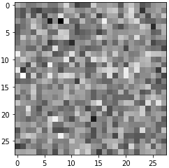
# Batch SIze만큼 노이즈 생성하여 그리드로 출력
rand = torch.randn(batch_size, 100, device=device)
img_1 = G(rand)
imshow_grid(img_1)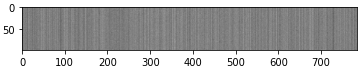
훈련
# Binary cross entropy loss and optimizer
criterion = nn.BCELoss()
d_optimizer = torch.optim.Adam(D.parameters(), lr=0.0002)
g_optimizer = torch.optim.Adam(G.parameters(), lr=0.0002)
def denorm(x):
out = (x + 1) / 2
return out.clamp(0, 1)
def reset_grad(): # 가중치를 0으로 초기화
d_optimizer.zero_grad()
g_optimizer.zero_grad()dx_epoch = []
dgx_epoch = []
total_step = len(data_loader)
for epoch in range(num_epochs):
for i, (images, _) in enumerate(data_loader):
images = images.reshape(batch_size, -1).to(device)
# Create the labels which are later used as input for the BCE loss
real_labels = torch.ones(batch_size, 1).to(device)
fake_labels = torch.zeros(batch_size, 1).to(device)
# ================================================================== #
# Train the discriminator #
# ================================================================== #
# Compute BCE_Loss using real images where BCE_Loss(x, y): - y * log(D(x)) - (1-y) * log(1 - D(x))
# Second term of the loss is always zero since real_labels == 1
outputs = D(images)
d_loss_real = criterion(outputs, real_labels)
real_score = outputs
# Compute BCELoss using fake images
# First term of the loss is always zero since fake_labels == 0
z = torch.randn(batch_size, latent_size).to(device)
fake_images = G(z)
outputs = D(fake_images)
d_loss_fake = criterion(outputs, fake_labels)
fake_score = outputs
# Backprop and optimize
d_loss = d_loss_real + d_loss_fake
reset_grad()
d_loss.backward()
d_optimizer.step()
# ================================================================== #
# Train the generator #
# ================================================================== #
# Compute loss with fake images
z = torch.randn(batch_size, latent_size).to(device)
fake_images = G(z)
outputs = D(fake_images)
g_loss = criterion(outputs, real_labels)
# Backprop and optimize
reset_grad()
g_loss.backward()
g_optimizer.step()
if (i+1) % 200 == 0:
print('Epoch [{}/{}], Step [{}/{}], d_loss: {:.4f}, g_loss: {:.4f}, D(x): {:.2f}, D(G(z)): {:.2f}'
.format(epoch, num_epochs, i+1, total_step, d_loss.item(), g_loss.item(),
real_score.mean().item(), fake_score.mean().item()))
dx_epoch.append(real_score.mean().item())
dgx_epoch.append(fake_score.mean().item())
# real image 저장
if (epoch+1) == 1:
images = images.reshape(images.size(0), 1, 28, 28)
save_image(denorm(images), os.path.join(sample_dir, 'real_images.png'))
# 생성된 이미지 저장
fake_images = fake_images.reshape(fake_images.size(0), 1, 28, 28)
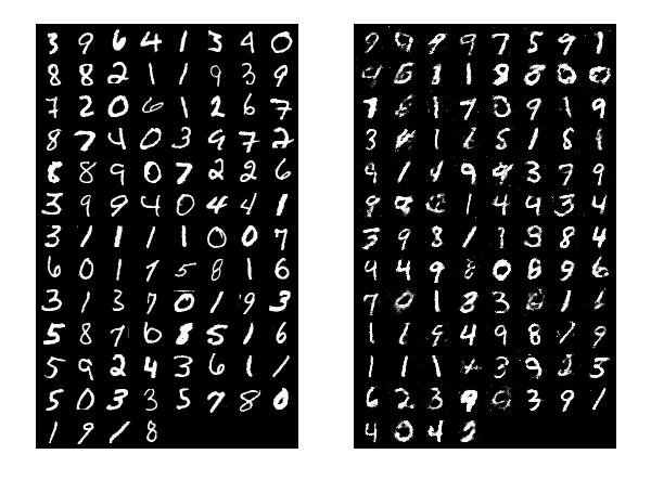
save_image(denorm(fake_images), os.path.join(sample_dir, 'fake_images-{}.png'.format(epoch+1)))
# 생성자, 판별자 각각 모델 저장
torch.save(G.state_dict(), 'G.ckpt')
torch.save(D.state_dict(), 'D.ckpt')
결과 확인
# plot
plt.figure(figsize = (12, 8))
plt.xlabel('epoch')
plt.ylabel('score')
x = np.arange(num_epochs)
plt.plot(x, dx_epoch, 'g', label='D(x)')
plt.plot(x, dgx_epoch, 'b', label='D(G(z))')
plt.legend()
plt.show()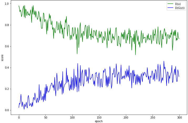
참고자료
반응형
'머신러닝, 딥러닝 ML, DL > Pytorch' 카테고리의 다른 글
| [Pytorch] Autograd, 자동 미분 ( requires_grad, backward(), 예시 ) (2) | 2021.10.02 |
|---|---|
| [Pytorch] 파이토치, 선형 회귀(Linear Regression) 간단히 구현해보기 (2) | 2021.09.24 |
| [Pytorch] 파이토치, 텐서(Tensor)란 (텐서 속성, 텐서 초기화) (0) | 2021.09.24 |